
Overview
This case study illustrates an investigation involving more than one metric. In typical performance investigations, you will need to peel out multiple layers of the stack in order to observe the component causing the actual performance pathology. This case study specifically examines sluggish application performance caused due to slow IO responses from the disk subsystem. This example will demonstrate a technique of looking at the performance of each layer in the I/O stack to find which layer is responsible for the most latency, then looking for constrained resources that the layer might need to access. This technique is valuable for finding the most-constrained resource in the system, potentially giving actionable information about resources that can be expanded to increase performance.
For the following example, we will inspect latency at two layers: the Network File System (NFS) layer on the Delphix Engine, and the disk layer below it. Both of these layers provide the latency axis, which gives a histogram of wait times for the clients of each layer.
Investigation
The analytics infrastructure enables users to observe the latency of multiple layers of the software stack. This investigation will examine the latency of both layers, and then draw conclusions about the differences between the two.
Setup
To measure this data, create two slices. When attempting to correlate data between two different statistics, it can be easier to determine causation when collecting data at a relatively high frequency. The fastest that each of these statistics will collect data is once per second, so that is the value used.
-
A slice collecting the latency axis for the statistic type NFS_OPS.
/analytics create set name=slice1 set statisticType=NFS_OPS set collectionInterval=1 set collectionAxes=latency commit -
A slice collecting the latency axis for the statistic type DISK_OPS.
/analytics

create
set name=slice2
set statisticType=DISK_OPS
set collectionInterval=1
set collectionAxes=latency
commit
After a short period of time, read the data from the first statistic slice.
select slice2
getData
setopt format=json
commit
setopt format=text
The same process works for the second slice. The setopt steps allow you to see the output better via the CLI. The output for the first slice might look like this:
{
    "type": "DatapointSet",
    "collectionEvents": [],
    "datapointStreams": [{
        "type": "NfsOpsDatapointStream",
        "datapoints": [{
            "type": "IoOpsDatapoint",
            "latency": {
                "512": "100",
                "1024": "308",
                "2048": "901",
                "4096": "10159",
                "8192": "2720",
                "16384": "642",
                "32768": "270",
                "65536": "50",
                "131072": "11",
                "524288": "64",
                "1048576": "102",
                "2097152": "197",
                "4194304": "415",
                "8388608": "320",
                "16777216": "50",
                "33554432": "20",
                "67108864": "9",
                "268435456": "2"
            },
            "timestamp": "2013-05-14T15:51:40.000Z"
        }, {
            "type": "IoOpsDatapoint",
            "latency": {
                "512": "55",
                "1024": "130",
                "2048": "720",
                "4096": "6500",
                "8192": "1598",
                "16384": "331",
                "32768": "327",
                "65536": "40",
                "131072": "14",
                "262144": "87",
                "524288": "42",
                "1048576": "97",
                "2097152": "662",
                "4194304": "345",
                "8388608": "280",
                "16777216": "22",
                "33554432": "15",
                "134217728": "1"
            },
            "timestamp": "2013-05-14T15:51:41.000Z"
        }, ...]
    }],
    "resolution": 1
}
For the second slice, it might look like this:
{
    "type": "DatapointSet",
    "collectionEvents": [],
    "datapointStreams": [{
        "type": "DiskOpsDatapointStream",
        "datapoints": [{
            "type": "IoOpsDatapoint",
            "latency": {
                "262144": "1",
                "524288": "11",
                "1048576": "13",
                "2097152": "34",
                "4194304": "7",
                "8388608": "2",
                "16777216": "3",
                "33554432": "1"
            },
            "timestamp": "2013-05-14T15:51:40.000Z"
        }, {
            "type": "IoOpsDatapoint",
            "latency": {
                "262144", "5",
                "524288", "10",
                "1048576", "14",
                "2097152", "26",
                "4194304", "7",
                "8388608", "4",
                "16777216", "2"
            },
            "timestamp": "2013-05-14T15:51:41.000Z"
        }, ...]
    }],
    "resolution": 1
}
The data is returned as a set of datapoint streams. Streams hold the fields that would otherwise be shared by all the datapoints they contain, but only one is used in this example because there are no such fields. Streams are discussed in more detail in the Performance Analytics Tool Overview. The resolution field indicates how many seconds each datapoint corresponds to, which in our case matches the requested collectionInterval. The collectionEvents field is not used in this example, but lists when the slice was paused and resumed to distinguish between moments when no data was collected because the slice was paused, and moments when there was no data to collect.
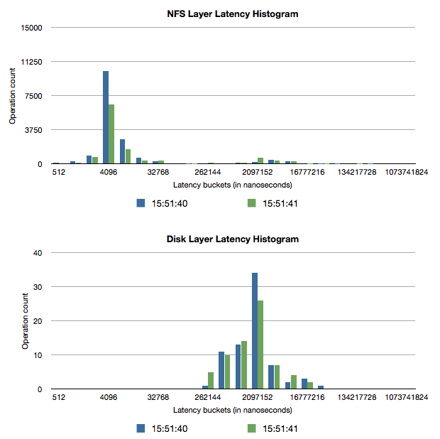
Graphically, these four histograms across two seconds look like this:
Analysis
Because the NFS layer sits above the disk layer, all NFS operations that use the disk synchronously (synchronous writes and uncached reads) will have latencies that are slightly higher than those of their corresponding disk operations. Usually, because disks have very high seek times compared to the time the NFS server spends on CPU, disk operations are responsible for almost all of the latency of these NFS operations. In the graphical representation, you can see this by looking at how the slower cluster of NFS latencies (around 2ms-8ms) have similar latencies to the median of the disk I/O (around 2ms-4ms). Another discrepancy between the two plots is that the number of disk operations is much lower than the corresponding number of NFS operations. This is because the Delphix filesystem batches together write operations to improve performance.
If database performance is not satisfactory and almost all of the NFS operation time is spent waiting for the disks, it suggests that the disk is the slowest piece of the I/O stack. In this case, disk resources (the number of IOPS to the disks, the free space on the disks, and the disk throughput) should be investigated more thoroughly to determine if adding more capacity or a faster disk would improve performance. However, care must be taken when arriving at these conclusions, as a shortage of memory or a recently-rebooted machine can also cause the disk to be used more heavily due to fewer cache hits.
Sometimes, disk operations will not make up all of the latency, which suggests that something between the NFS server and the disk (namely, something in the Delphix Engine) is taking a long time to complete its work. If this is the case, it is valuable to check whether the Delphix Engine is resource-constrained, and the most common areas of constraint internal to the Delphix Engine are CPU and memory. If either of those is too limited, you should investigate whether expanding the resource would improve performance. If no resources appear to be constrained or more investigation is necessary to convince you that adding resources would help the issue, Delphix Support is available to help debug these issues.
While using this technique, you should take care to recognize the limitations that caching places on how performance data can be interpreted. In this example, the Delphix Engine uses a caching layer for the data it stores, so asynchronous NFS writes will not go to disk quickly because they are being queued into larger batches, and cached NFS reads won't use the disk at all. This causes these types of NFS operations to return much more quickly than any disk operations are able to, resulting in a very large number of low-latency NFS operations in the graph above. For this reason, caching typically creates a bimodal distribution in the NFS latency histograms, where the first cluster of latencies is associated with operations that only hit the cache, and the second cluster of latencies is associated with fully or partially uncached operations. In this case, cached NFS operations should not be compared to the disk latencies because they are unrelated. It is possible to use techniques described in the first example to filter out some of the unrelated operations to allow a more accurate mapping between disk and NFS latencies.
-
Begin the performance investigation by examining some high-level statistics such as latency.
-
Create a slice with statistic type NFS_OPS.
-
Set the slice to collect the latency axis.
-
Do not add any constraints.
-
Set the collection interval. Anything over one second will work, but ten seconds gives good data resolution and will not use a lot of storage to persist the data that is collected. The rest of this example will assume a collection period of ten seconds for all other slices, but any value could be used.
/analytics

create
set name=step1
set statisticType=NFS_OPS
set collectionInterval=10
set collectionAxes=latency
commit
This will collect a time series of histograms describing NFS latencies as measured from inside the Delphix Engine, where each histogram shows how many NFS I/O operations fell into each latency bucket during every ten-second interval. After a short period of time, read the data from the statistic slice:
select step1
getData
setopt format=json
commit
setopt format=text
The
setoptsteps are optional but allow you to see the output better via the CLI. The output looks like this:{ "type": "DatapointSet", "collectionEvents": [], "datapointStreams": [{ "type": "NfsOpsDatapointStream", "datapoints": [{ "type": "IoOpsDatapoint", "latency": { "32768": "16", "65536": "10" }, "timestamp": "2013-05-14T15:51:40.000Z" }, ...] }], "resolution": 10 }The data is returned as a set of datapoint streams. Streams hold the fields which are shared by all the data points they contain. Later on, in this example, the opt and client fields will be added to the streams, and multiple streams will be returned. Streams are described in more detail in Performance Analytics Tool Overview. The
resolutionfield indicates the number of seconds that corresponds to each datapoint, which in our case matches the requestedcollectionInterval. ThecollectionEventsthe field is not used in this example, but lists when the slice was paused and resumed, to distinguish between moments when no data was collected because the slice was paused, and moments when there was no data to collect.
-
-
If the latency distributions show some slow NFS operations, the next step would be to determine whether the slow operations are reads or write.
-
Specify a new NFS_OPS slice to collect this by collecting the op and latency axes.
-
To limit output to the long-running operations, create a constraint on the latencyaxis that prohibits the collection of data on operations with latency less than 100ms.
/analytics

create
set name=step2
set statisticType=NFS_OPS
set collectionInterval=10
set collectionAxes=op,latency

edit axisConstraints.0
set axisName=latency
set type=IntegerGreaterThanConstraint
set greaterThan=100000000
back

commit
The
greaterThanthe field is 100ms converted into nanoseconds.Reading the data proceeds in the same way as the first step, but there will be two streams of data points, one where
op=write,and one whereop=read.Info : Because we constrained output to operations with latencies higher than 100ms, none of the latency histograms will all have any buckets for latencies lower than 100ms.
-
-
After inspecting the two data streams, you might find that almost all slow operations are writes, so it could be valuable to determine which clients are requesting the slow writes, and how large each of the writes is.
-
To collect this data, create a new NFS_OPS slice which collects the size and client axes.
-
Add constraints ensuring that the op axis should be constrained to only collect data for write operations, and the latencyaxis should be constrained to filter operations taking less than 100ms. Info: Because the constraint on the op axis dictates that it will always have the value write, it is not necessary to collect the op axis anymore.
/analytics

create
set name=step3
set statisticType=NFS_OPS
set collectionInterval=10
set collectionAxes=size,client

edit axisConstraints.0
set type=IntegerGreaterThanConstraint
set axisName=latency
set greaterThan=100000000
back

edit EnumEqualConstraint
set type=StringEqualConstraint
set axisName=op
set equals=write
back

commit
Reading the data proceeds in the same way as the first two steps, but there will be one stream for every NFS client. The dataset collected by this will consist of a set of streams, one corresponding to each NFS client, and each stream will be a time series of histograms showing write sizes that occurred during each ten-second interval.
Continuing to use this approach will allow you to narrow down the slow writes to a particular NFS client, and you may be able to tune that client in some way to speed it up.
-